Evolutionary game analysis on the regulation of medical devices used in health services delivery

Table of Contents

Strategy stability analysis of MDs enterprise

Based on the payoff matrix, the expected returns of MDs enterprise supplying high or low quality MDs are as follows respectively.

$$U11=[yz+y(1-z)+(1-y)z+(1-y)(1-z)](Re0-Ce1)$$

(1)

$$\begingathered U12 = yz\left( Re0 – Ce2 – Pe1 – Pe2 \right) + y\left( 1 – z \right)\left( Re0 – Ce2 – Pe1 – aPe2 \right) \hfill \\ \quad \quad \quad + \left( 1 – y \right)z\left( Re0 – Ce2 – Pe2 \right) + \left( 1 – y \right)\left( 1 – z \right)\left(Re0 – Ce2 – aPe2 \right) \hfill \\ \endgathered$$

(2)

And the average expected return of MDs enterprise is

The replication dynamic equation of strategy selection for MDs enterprise can be expressed as

$$F(x)= \fracdxdt =x(U11-U1)=x(1-x)(Ce2-Ce1+aPe2+yPe1+zPe2-azPe2)$$

(4)

The first order derivative of $x$ is

$$\fracdF(x)dx=(1-2x)(Ce2-Ce1+aPe2+yPe1+zPe2-azPe2)$$

(5)

According to the stability principle of differential equation, the condition of MDs enterprise selecting stable strategy is $F(x)=0$ and $\fracdF(x) dx<0$.

If $F(x)=0$, there are three solutions:

$$x1=0, x2=0, y1=-(Ce2-Ce1+aPe2+zPe2-azPe2)/Pe1$$

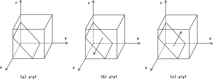
When $y=y1$, $\fracdF(x)dx=0$, then $x$ is always in a stable state.
When $y>y1$, $\fracdF(0)dx>0$, $\fracdF(1)dx<0$, then $x=1$ is an evolutionarily stable strategy (ESS).
When $y<y1$, $\fracdF(0)dx<0$, $\fracdF(1)dx>0$, then $x=0$ is an ESS.

Phase diagram of MDs enterprise strategy evolution is depicted in Fig. 2.

Strategy stability analysis of hospital

Based on the payoff matrix, for the hospital, the expected return of selecting “conduct strict management” is

$$U21=xz(-Ch1)+x(1-z)(-Ch1)+(1-x)z(-Ch1-Ch2)+(1-x)(1-z)(-Ch1-Ch2)$$

(6)

The expected return of the choosing “conduct loose management” is

$$U22=xz(-Ph1)+x(1-z)(-bPh1)+(1-x)z(-Ph1-Ch2)+(1-x)(1-z)(-bPh1-Ch2)$$

(7)

Thus, the average expected return of hospital strategy selection is

$$U2 =yU21+\left(1-y\right)U22$$

(8)

The replication dynamic equation for hospital strategy selection is

$$F(y)= \fracdydt =y(U21-U22)=y(1-y)(bPh1-Ch1+zPh1-bzPh1)$$

(9)

The first order derivative of $y$ is

$$\fracdF(y)dy=(1-2y)(bPh1-Ch1+zPh1-bzPh1)$$

(10)

According to the differential equation stability principle, the condition of hospital selecting stable strategy is $F(y)=0$ and $\fracdF(y) dy<0$.

If $F(y)=0$, there are three solutions:

$$y1=0, y2=1, z1=(Ch1-bPh1)/(Ph1-bPh1)$$

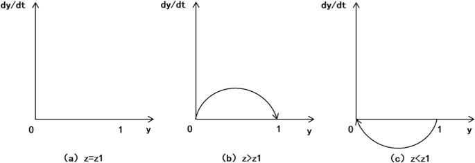
When $z=z1$, $\fracdF(y)dy=0$, then $y$ is always in a stable state.
When $z>z1$, $\fracdF(0)dy>0$, $\fracdF(1)dy<0$, then $y=1$ is an ESS.
When $z<z1$, $\fracdF(0)dy<0$, $\fracdF(1)dy>0$, then $y=0$ is an ESS.

Phase diagram of hospital strategy evolution is shown in Fig. 3.

Strategy stability analysis of government

From the payoff matrix, the expected returns of government selecting “perform active regulation” and “perform passive regulation” can be marked as $U31$ and $U32$

$$\begingathered U31 = xy\left( G + Rg1 – Cg1 \right) + x\left( 1 – y \right)\left( G + Ph1 – Cg1 \right) + \left( 1 – x \right)y\left( G + Pe2 \right) \hfill \\ \quad \quad \quad + \left( 1 – x \right)\left( 1 – y \right)\left( G + Pe2 + Ph1 + Cg1 – Cg2 \right) \hfill \\ \endgathered$$

(11)

$$\begingathered U32 = xy\left( Rg1 \right) + x\left( 1 – y \right)\left( bPh1 – S2 \right) + \left( 1 – x \right)y\left( aPe2 – S1 \right) \hfill \\ \quad \quad \quad + \left( 1 – x \right)\left( 1 – y \right)\left( aPe2 + bPh1 – S1 – S2 – Cg2 \right) \hfill \\ \endgathered$$

(12)

So, the average expected return of government strategy selection can be expressed as

$$U3 =zU31+\left(1-z\right)U32$$

(13)

The replication dynamic equation for government strategy selection is

$$\begingathered F\left( z \right) = \fracdzdt = z\left( U31 – U32 \right) = z\left( 1 – z \right)\left( Cg1 + G + Pe2 + Ph1 + S1 + S2 – aPe2 \right. \hfill \\ \quad \quad \quad – bPh1 – 2xCg1 – yCg1 – xPe2 – yPh1 – xS1 \hfill \\ \left. \quad \quad \quad – yS2 + azPe2 + byPh1 + xyCg1 \right) \hfill \\ \endgathered$$

(14)

The first order derivative of $z$ is

$$\begingathered \fracdF\left( z \right)dz = \left( 1 – 2z \right) \left[ Cg1\left( 1 – 2x – y + xy \right) + Pe2\left( 1 – a \right)\left( 1 – x \right) \right. \hfill \\ \left. \quad \quad \quad \quad + Ph1\left( 1 – b \right)\left( 1 – y \right) + G + S1\left( 1 – x \right) + S2\left( 1 – y \right) \right] \hfill \\ \endgathered$$

(15)

According to the differential equation stability principle, the condition of government selecting stable strategy is $F(z)=0$ and $\fracdF(z) dz<0$.

If $F(z)=0$, there are three solutions:

$$\begingathered z1 = 0, z2 = 1, \hfill \\ x1 = – \left[ G + S1 + \left( 1 – a \right)Pe2 + \left( 1 – y \right) Cg1 + \left( 1 – y \right)S2 + \left( 1 – b \right)\left( 1 – y \right) Ph1 \right] \hfill \\ \quad \quad\;/\left[ \left( y – 2 \right)Cg1 – S1 – \left( 1 – a \right)Pe2 \right] \hfill \\ \endgathered$$
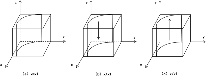
When $x=x1$, $\fracdF(z)dz=0$, then $z$ is always in a stable state.
When $x>x1$, $\fracdF(0)dz<0$, $\fracdF(1)dz>0$, then $z=0$ is an ESS.
When $x<x1$, $\fracdF(0)dz>0$, $\fracdF(1)dz<0$, then $z=1$ is an ESS.

Phase diagram of government strategy evolution is shown in Fig. 4.

Strategy stability analysis of tripartite evolutionary game

The equilibrium points can be calculated if $F(x)=0$, $F(y)=0$, and $F(z)=0$. According to the Eqs. (4), (9) and (14), 8 pure strategy Nash equilibrium points can be obtained: $E1(\text0,0,0)$, $E2(\text1,0,0)$, $E3(\text0,1,0)$, $E4(\text0,0,1)$, $E5(\text1,1,0)$, $E6(\text1,0,1)$, $E7(\text0,1,1)$, $E8(\text1,1,1)$.

The Jacobian matrix of the tripartite evolutionary game system is

$$J = \left[\beginarraycccJ11& J12& J13\\ J21& J22& J23\\ J31& J32& J33\endarray\right] = \left[\beginarrayccc\textdF(\textx)/\textdx& \textdF(\textx)/\textdy& \textdF(\textx)/\textdz\\ \textdF(\texty)/\textdx& \textdF(\texty)/\textdy& \textdF(\texty)/\textdz\\ \textdF(\textz)/\textdx& \textdF(\textz)/\textdy& \textdF(\textz)/\textdz\endarray\right]$$

where $J11$ to $J33$ can be expressed as as follows:

$$\begingathered J11 = \left( 1 – 2x \right)\left( Ce2 – Ce1 + aPe2 + yPe1 + zPe2 – azPe2 \right) \hfill \\ J12 = x\left( 1 – x \right)Pe1 \hfill \\ J13 = x\left( 1 – x \right)\left( 1 – a \right)Pe2 \hfill \\ J21 = 0 \hfill \\ J22 = \left( 1 – 2y \right)\left( bPh1 – Ch1 + zPh1 – bzPh1 \right) \hfill \\ J23 = y\left( 1 – y \right)\left( 1 – b \right)Ph1 \hfill \\ J31 = – z\left( 1 – z \right)\left( Cg1 + Pe2 + S1 – aPe2 – yCg1 + 1 \right) \hfill \\ J32 = – z\left( 1 – z \right)\left[ Cg1\left( 1 – x \right) + Ph1\left( 1 – b \right) + S2 \right] \hfill \\ J33 = \left( 1 – 2z \right)\left[ Cg1\left( 1 – 2x – y + xy \right) + Pe2\left( 1 – a \right)\left( 1 – x \right) \right. \hfill \\ \left. \quad \quad \quad + Ph1\left( 1 – b \right)\left( 1 – y \right) + G + S1\left( 1 – x \right) + S2\left( 1 – y \right) \right] \hfill \\ \endgathered$$

According to Lyapunov’s first method (indirect method), if all eigenvalues of the Jacobian matrix have negative real parts, the equilibrium point is asymptotically stable. If at least one of the eigenvalues of Jacobian matrix has a positive real part, the equilibrium point is an unstable point³⁰. We calculated the eigenvalue $\lambda 1$, $\lambda 2$ and $\lambda 3$ and analyzed the asymptotic stability condition of each equilibrium point (Table 3). For point $E1$, eigenvalue $\lambda 3=Cg1+G+Pe2(1-a)+Ph1(1-b)+S1+S2>0$, so $E1$ is an unstable point. For point $E3$, $\lambda 2=G+Pe2(1-a)+S1>0$, so $E3$ is an unstable point. Therefore, the remaining $E2(\text1,0,0)$, $E4(\text0,0,1)$, $E5(\text1,1,0)$, $E6(\text1,0,1)$, $E7(\text0,1,1)$, $E8(\text1,1,1)$ may be theoretically possible ESS.

Table 3 Eigenvalues and asymptotic stability conditions of equilibrium points.

Take equilibrium point $E5(1,1,0)$ as example, we prove its existence, local uniqueness, and analysis its stability conditions.

(1)

Existence of $E5$ equilibrium point

For $E5(1,1,0)$, we need to verify that it satisfies $F(x)=F(y)=F(z)=0$:

From $F(x)=x(1-x)[y(Pe1+Pe2)-Ce1+Ce2]=0$, at $\textx=1$, $\textF(\textx)=0$ is satisfied.
From $F(y)=y(1-y)[z(Ph1-bPh1)+bPh1-Ch1]=0$, at $y=1$, $F(y)=0$ is satisfied.
From $F(z)=z(1-z)[Cg1-G+x(Rg1-aPe2-Ph1)+y(Ph1-bPh1)] =0$, at $z=0$, $F(z)=0$ is satisfied.

Therefore, $E5(1,1,0)$ is indeed an equilibrium point of the model.

(2)

Local uniqueness analysis for $E5$

At $E5=(\text1,1,0)$, the partial derivatives are

$$\begingathered dF\left( x \right)/dx = Ce1 – Ce2 – Pe1 – aPe2 \hfill \\ dF\left( x \right)/dy = 0 \hfill \\ dF\left( x \right)/dz = 0 \hfill \\ dF\left( y \right)/dx = 0 \hfill \\ dF\left( y \right)/dy = Ch1 – bPh1 \hfill \\ dF\left( y \right)/dz = 0 \hfill \\ dF\left( z \right)/dx = 0 \hfill \\ dF\left( z \right)/dy = 0 \hfill \\ dF\left( z \right)/dz = G – Cg1 \hfill \\ \endgathered$$

Therefore, the Jacobian matrix $J(E5)$ is

$$\left[\beginarraycccCe1-Ce2-Pe1-aPe2 & 0& 0\\ 0& Ch1-bPh1& 0\\ 0& 0& G-Cg1\endarray\right]$$

The determinant of $J(E5)$ is

$$det(J) = (Ce1-Ce2-Pe1-aPe2)(Ch1-bPh1)(G-Cg1)$$

When $det(J)\ne 0$, by the implicit function theorem, $E5$ is locally unique.

(3)

Stability analysis for $E5$

Using Lyapunov’s first method, we analyze the eigenvalues of $J(E5)$:

$$\begingathered \lambda 1 = G – Cg1 \hfill \\ \lambda 2 = Ch1 – bPh1 \hfill \\ \lambda 3 = Ce1 – Ce2 – Pe1 – aPe2 \hfill \\ \endgathered$$

For $E5$ to be asymptotically stable, we need:

1)

$\lambda 1<0:G-Cg1<0$
2)

$\lambda 2<0:Ch1-bPh1<0$
3)

$\lambda 3<0:Ce1-Ce2-Pe1-aPe2<0$

These give the stability conditions for $E5$:

$Cg1>G$ (Government condition)
$Ch1<bPh1$ (Hospital condition)
$Ce1-Ce2<Pe1+aPe2$ (MDs enterprise condition)

These conditions can be interpreted in the following realistic ways:

1)

For government: When enterprises supplying high-quality products and hospitals implementing strict management, the cost of active regulation ($Cg1$) exceeds its social benefits ($G$), making passive regulation a more rational choice.
2)

For hospitals: The strict management cost ($Ch1$) must be less than the expected penalties ($bPh1$).
3)

For MDs enterprises: The cost difference between supply high and low quality MDs ($Ce1-Ce2$) must be less than the penalties and revenue loss ($Pe1+aPe2$).

Inference 1

The government’s regulatory strategy is influenced by the cost–benefit relationship of active regulation. When $Cg1>G$, indicating that regulation costs exceed the social benefits gained from active regulation, the government will tend toward passive regulation. Conversely, when $Cg1<G$, suggesting that the social benefits outweigh the costs of active regulation, the government will select active regulation strategy.

Inference 2

The equilibrium strategy of hospital depends on the relationship between punishment intensity and strict management costs. Specifically, when $Ch1>bPh1$, indicating that the expected punishment for loose management is less than the cost of conducting strict management, hospitals will stabilize at the loose management strategy. Conversely, if $Ch1<bPh1$, meaning that the expected punishment through whistleblowing exceeds the cost of implementing strict management, hospitals will choose strict management strategy.

Inference 3

The enterprise’s equilibrium strategy is determined by the balance between quality-related costs and potential penalties. When $Ce1-Ce2>Pe1+aPe2$, meaning the expected total punishment (penalties and revenue loss) is insufficient to offset the cost difference between supplying high and low quality products, MDs enterprise will choose to supply low-quality products. However, when $Ce1-Ce2<Pe1+aPe2$, indicating that the expected punishment through both direct regulation and whistleblowing exceeds the cost savings from supplying low-quality products, enterprise will select the strategy of supplying high-quality products.

link